Table of Contents
Introduction
In this tutorial we present two Poisson test problems, which demonstrate the multigrid behavior on a partially refined mesh. The examples are available in 2D and in 3D, see poisson_basic_2d.f90 and poisson_basic_3d.f90
Problem description
We use the method of manufactured solutions: from an analytic solution the right-hand side and boundary conditions are computed. The equation solved here is Poisson's equation with constant coefficients:
\[ \nabla^2 u = \nabla \cdot (\nabla u) = \rho , \]
in a rectangular domain of \([0,1]^D\), where \(D\) is the problem dimension.
We pick the following solution \(u\)
\[ u(r) = \exp(|{\vec{r}-\vec{r}_1}|/\sigma) + \exp(|{\vec{r}-\vec{r}_2}|/\sigma), \]
where \(\vec{r_1} = (0.25, 0.25)\), \(\vec{r_2} = (0.75, 0.75)\) (2D) and \(\vec{r_1} = (0.25, 0.25, 0.25)\), \(\vec{r_2} = (0.75, 0.75, 0.75)\) (3D) and \(\sigma = 0.04\). An analytic expression for the right-hand side \(\rho\) is obtained by plugging the solution into the original equation.
Explanation of example
In the code, the solution is stored used the module m_gaussians. This module also contains the type m_gaussians::gauss_t and the subroutine m_gaussians::gauss_init() to initialize it as follows:
The variable tree contains the full AMR mesh. It is of type a2_t, and a call to m_a2_core::a2_init() takes care of the initialization:
We define box_size = 8, which means that each box has \( 8 \times 8\) cells, and dr = 0.125 (so that the domain length is one). The variable n_var_cell, the number of cell centered values, is set to 4 (reserved for i_phi, i_rhs, i_err and i_tmp, see below), whereas the variable n_var_face, the number of face centered values, is zero.
In Afivo the coarsest mesh, which covers the full computational domain, is not supposed to change. To create this mesh there is a routine a2_set_base(), which takes as input the spatial indices of the coarse boxes and their neighbors. Below, a 2D example is shown for creating a single coarse box at index \((1,1)\). Physical (non-periodic) boundaries are indicated by a negative index for the neighbor. By adjusting the neighbors one can specify different geometries, the possibilities include meshes that contain a hole, or meshes that consist of two isolated parts. The treatment of boundary conditions is discussed in Filling ghost cells
The routine m_a2_types::a2_print_info shows some values of the tree. At this position in the example, it lists:
*** a2_print_info(tree) ***
Current maximum level:           1
Maximum allowed level:          30
Number of boxes used:            3
Memory limit(boxes):       4793490
Memory limit(GByte):      0.16E+02
Highest id in box list:          3
Size of box list:             1000
Box size (cells):                8
Number of cc variables:          4
Number of fc variables:          0
Type of coordinates:             0
min. coords:          0.0000E+00  0.0000E+00
dx at min/max level   0.1250E+00  0.1250E+00
Note that the number of boxes is 3, although the maximum multigrid level is just 1. This arises from the fact that for multigrid cycling also a level 0 of box size \( 4 \times 4 \), and a level -1 have been defined of size \( 2 \times 2 \). The memory limit has been set on 16 GB (default value) which results in at most 4793490 boxes, based on the box size and the number of ghost cells in each direction (i.e., 2) and the numbers of cell and face centered variables. The length of the box list is 1000, but if more boxes are required, the length will be extended and boxes which are not longer used will be cleaned up. Since box_size = 8 this implies that each box has \( 8 \times 8\) cells, excluding ghost cells, and, since the problem is solved on a rectangular domain of \([0,1] \times [0,1]\), (min. coords: 0.0000E+00 0.0000E+00, the cell size dx at the coarsest level is dr = 1 / 8.
Next, we start refining the mesh by means of subroutine refine_routine which has been added to the example poisson_basic_2d.f90
Here variable id denotes the index number of the box. m_a2_types::a2_r_cc is one of those useful features from module m_a2_types to calculate the center of a cell. The refinement is based on the fourth derivative of the solution. This example only shows when a box should be refined or not, the derefinement does not play a role here. Besides, value af_do_ref, indicating you want to refine a box, the value af_keep_ref, indicating you want to keep a box's refinement, and af_rm_ref, indicating you want to derefine a box, are available. The routine m_a2_core::a2_adjust_refinement ensures the 2:1 balance is ensured, so that there is never a jump of more than one refinement level between neighboring boxes. These constraints are automatically handled, so that the user-defined refinement function does not need to impose them.
When boxes are added or removed in the refinement procedure, their connectivity is automatically updated. References to a removed box are removed from its parent and neighbors. When a new box is added, its neighbors are found through its parent. Three scenarios can occur: the neighbor can be one of the other children of the parent, the neighbor can be a child from the neighbor of the parent, or the neighbor does not exist. In the latter case, there is a refinement boundary, which is indicated by the special value m_afivo_types::af_no_box.
In the next loop, first the routine m_a2_utils::a2_loop_box is called for each box, with as argument the user-defined routine
which calls gauss_laplacian from m_gaussian corresponding the problem described above. The routine a2_r_cc computes the cell center of the cells in the box. In this example, each box has 4 cell centered matrices. Here boxcc(:,:,i_rhs) is initialized with the right hand side values.
The following do loop all right hand side field of the boxed used are initialized and boxes are refined in accordance with the refinement routine to obtain an adaptive mesh.
If no further refinement is required, i.e., refine_info\n_add == 0, the do loop stops.
The routine m_a2_types::a2_print_info shows after the refinement loop:
 *** a2_print_info(tree) ***
 Current maximum level:          10
 Maximum allowed level:          30
 Number of boxes used:         5487
 Memory limit(boxes):       4793490
 Memory limit(GByte):      0.16E+02
 Highest id in box list:       5487
 Size of box list:             8030
 Box size (cells):                8
 Number of cc variables:          4
 Number of fc variables:          0
 Type of coordinates:             0
 min. coords:          0.0000E+00  0.0000E+00
 dx at min/max level   0.1250E+00  0.2441E-03
So ten levels of refinement are required leading to 5487 boxes and a cell size of the highest level of \(1 / 4096\).
Viewing results
By means of a call to a2_write_vtk from module m_a2_output a vtu file can be produced to show the adapted mesh, but also the solution.
The resulting file "poisson_basic_2d_0.vtu" in directory output can be viewed by Visit.
| a | b |
|---|---|
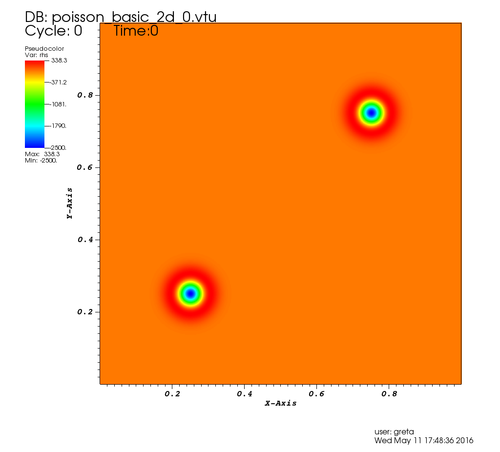
a | 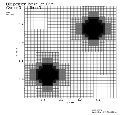
b |
Figure 1. a) initialization of the right hand side b) adapted mesh
Now the grid has been constructed to match the RHS function and in accordance with the refinement function refine_routine showed above, we continue to solve the Poisson problem using multigrid. Therefore we first initialize the multigrid options. The routine m_a2_multigrid::mg2_init performs some basic checks and sets default values where necessary in variable mg of type m_a2_multigrid::mg2_t.
To this end, we perform a number of multi-grid iterations. Within each loop we call routine m_a2_multigrid::mg2_fas_fmg, performing a full approximation scheme using full multigrid. At the first call of mg2_fas_fmg sets the initial guess for phi and restricts the right hand side fields rhs from the highest level down to the coarsest level. After the first call of mg2_fas_fmg it sets the right hand side field on coarser grids and restricts the field with the holding solution of phi. If required the ghost cells are filled.
Next the user-defined routine set_error is called to computed the error compared to the analytic solution.
The results of the first 10 iterations steps are listed below:
Multigrid iteration | max residual | max error
      1                1.00579E+01   5.13811E-05
      2                4.54153E-01   5.13903E-05
      3                2.26078E-02   5.13902E-05
      4                1.14302E-03   5.13902E-05
      5                5.79126E-05   5.13902E-05
      6                2.94218E-06   5.13902E-05
      7                1.50202E-07   5.13902E-05
      8                2.38767E-08   5.13902E-05
      9                2.36430E-08   5.13902E-05
     10                2.01674E-08   5.13902E-05
Note that the residual is still decreasing, whereas the maximum error reaches its minimum after about three iterations.
After 10 multigrid iterations we obtain the resulting file "poisson_basic_2d_10.vtu" in directory output, which can be viewed by e.g., visit.
| Solution \( \phi \) | Error \( \epsilon \) after 10 multigrid iteration steps |
|---|---|
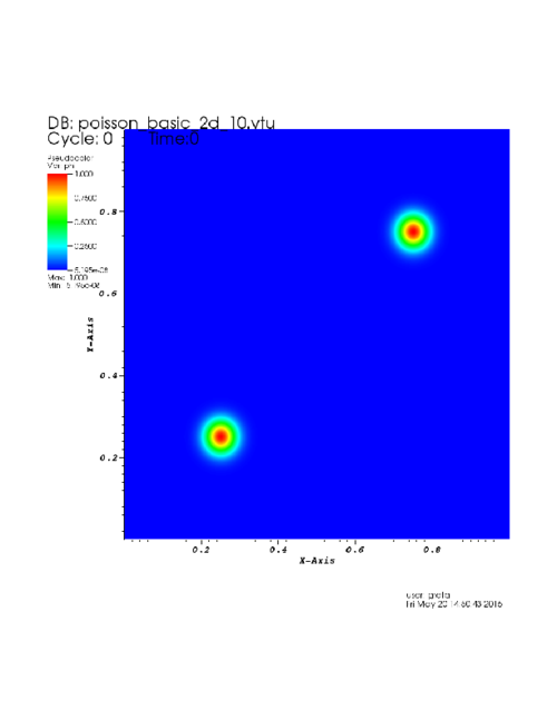
a | 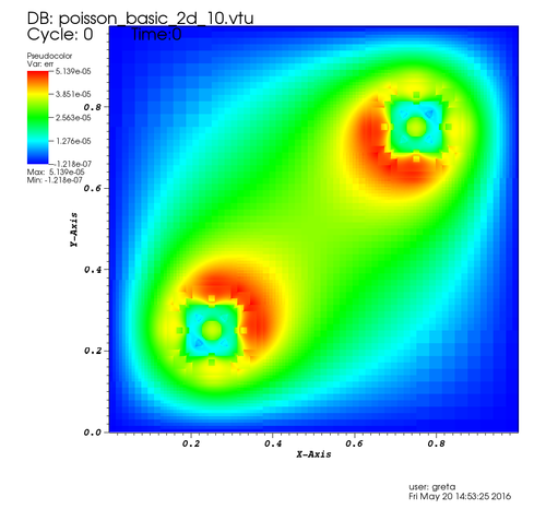
b |
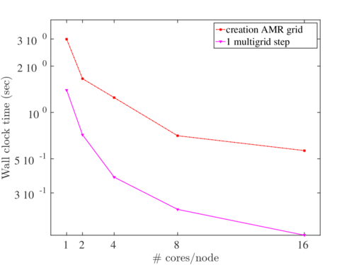
Parallel results
The info below is coming from the corresponding 3d problem for boxes of size \(8 \times 8 \times 8\), excluding ghost cells.
*** a3_print_info(tree) ***
Current maximum level:           9
Maximum allowed level:          30
Number of boxes used:         8811
Memory limit(boxes):        525314
Memory limit(GByte):      0.16E+02
Highest id in box list:       8811
Size of box list:            12502
Box size (cells):                8
Number of cc variables:          4
Number of fc variables:          0
Type of coordinates:             0
min. coords:          0.0000E+00  0.0000E+00  0.0000E+00
dx at min/max level   0.1250E+00  0.4883E-03
On the coarsest level the variable \(dx = 1 / 8\), the size of a cell, whereas on the highest level \(dx = 1 / 2048\). We have compared, for this 3D case, the wall clock time, obtained by a calculation with just one thread and with multiple threads. This shows that the use of OpenMP is very succesful. We distinguish the wall clock time for both the creation of the adaptive mesh refinement part of the program and the multigrid process. For the adaptive mesh refinement part, we obtain a factor of 5.3, comparing the wall clock time for 16 and just one thread. For the multigrid process we achieve a speedup factor of nearly a factor 9.